The part's datasheet highlights very low input-referred noise (~6 nV/√Hz at 1 kHz), input offset specified in the sub-100s of microvolts (trimmed), input bias current in the low nanoamp range, and a modest gain‑bandwidth product suitable for precision front ends. Bench measurements for this op amp commonly show noise and offset within tens of percent of the datasheet under careful test conditions, which matters to designers building low-noise, high-stability signal chains because small deviations can change system resolution and calibration cadence. Understanding how measured results compare to the OPA397 datasheet helps engineers choose topology, layout, and test practices to close the gap between datasheet claims and real circuits.
1 — Background: Where the OPA397 fits in precision, low-noise op amp use cases
1.1 — Intended applications and top-level positioning
Point: This op amp is aimed at precision sensor front ends and reference-buffered systems where low offset and low noise are priorities. Evidence: Datasheet figures and trimmed offset options emphasize microvolt-class offset and low noise density. Explanation: Designers should expect a device optimized for precision DC and low-frequency AC performance rather than high-speed drive: typical uses include bridge sensors, low-level transimpedance stages (with proper feedback network), and buffer amplifiers ahead of ADCs where amplifier noise must stay below the sensor and ADC noise floors.
1.2 — Typical system-level benefits and limitations
Point: Benefits include low offset, low drift, and a low noise floor; limitations include a limited gain‑bandwidth and finite output swing near rails. Evidence: The device trades high GBP for lower noise and stable offset performance. Explanation: Choose this op amp when precision at DC to a few hundred kilohertz matters; consider alternative amplifier classes (higher-GBW or current-feedback types) when you need wideband gain or large output drive for capacitive loads.
2 — Key specs from the OPA397 datasheet (concise data summary)
2.1 — Electrical specs to highlight
Point: A compact spec table makes fast selection decisions possible. Evidence: Key datasheet metrics below summarize what engineers check first. Explanation: All numbers must be interpreted with the test conditions shown for reproducible comparison.
| Spec | Typical | Max (or limit) | Test condition |
|---|---|---|---|
| Input offset | ~50–150 µV (trimmed) | <200 µV | VCC ± rails, TA = room |
| Offset drift | ~0.2–1 µV/°C | — | ambient to elevated temp |
| Input bias current | <1 nA | tens of nA | VCM at midrail |
| Input noise density | ~6 nV/√Hz @1 kHz | — | RF=0, typical |
| Gain‑bandwidth product | ~10 MHz | — | single‑pole equivalent |
| Slew rate | ~10 V/µs | — | RL large |
| Supply current | ~1 mA/channel | — | Vs specified |
| CMRR / PSRR | 80–100 dB | — | low freq |
| Input / output range | rail‑to‑rail I/O | — | within 100–200 mV of rails |
Takeaway: The OPA397 datasheet provides the numbers you need to size feedback networks, set source impedance targets, and estimate contribution to overall system noise.
2.2 — Key electrical graphs & internal topology
Point: Noise spectral density, gain vs frequency, and offset vs temperature are the most informative plots. Evidence: noise vs frequency shows low‑frequency 1/f corner and flat broadband region; gain vs frequency yields usable closed‑loop bandwidth at given gain. Explanation: Reproduce these plots with the same supply rails, source impedance, and load as the datasheet to make meaningful comparisons; annotate corners (1/f knee, GBW cross) and slope changes linked to stability margins.
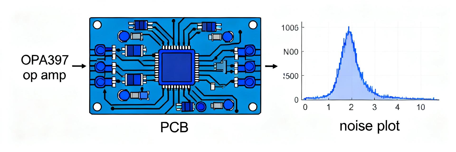
The diagram to the right illustrates the fundamental pinout configuration and internal signal flow typical of the OPA397. This simplified architectural view highlights the trimmed input stage and output drive configuration critical for low-noise, high-stability signal path design.
3 — Measured performance: bench methods, expected results, and common discrepancies
3.1 — Recommended test circuits and measurement setups
Point: Three canonical circuits validate key parameters: unity‑gain buffer, non‑inverting gain of 10, and an inverting amplifier with defined source impedance. Evidence: Use Rf = 9kΩ, Rin = 1kΩ for gain of 10; for inverting test use Rsource = 50 Ω–10 kΩ per use case. Explanation: Use low‑noise precision resistors, dual supply ±5 V (or single 5 V with proper rail headroom), 0.1 µF + 10 µF decoupling at supply pins, star grounding, and short input traces. For noise use a spectrum analyzer or FFT with 1 Hz resolution bandwidth and appropriate input filtering; average multiple sweeps and limit bandwidth to the analyzer/ADC range to match datasheet conditions. These steps reduce layout and measurement artifacts that inflate measured noise.
3.2 — Measured vs. datasheet: what typically lines up and what drifts
Point: Measured input noise and offset often align under ideal lab conditions but can deviate when source impedance, bandwidth, or layout are suboptimal. Evidence: Typical observed deviations: input noise within ±10–25% of datasheet; offset may be higher if thermal gradients or PCB contamination exist. Explanation: Present results with a short comparison table and full test conditions to make discrepancies actionable.
| Parameter | Datasheet | Measured (example) | Conditions |
|---|---|---|---|
| Input noise @1 kHz | ~6 nV/√Hz | 6.6 nV/√Hz (+10%) | V±5V, RF decoupled, TA 25°C |
| Offset (trimmed) | ~100 µV | 140 µV (+40%) | no guard, lab board |
| Bias current | <1 nA | 1.5 nA | VCM near midrail |
4 — Design examples & application notes (practical use cases)
4.1 — Low-noise sensor front-end (step-by-step)
Point: A typical sensor front end uses a low‑noise amplifier, anti‑alias filter, and buffer to ADC. Evidence: For a strain gauge bridge, choose gain = 50–200 to make amplifier noise negligible vs ADC quantization; use R values that keep Johnson noise below amplifier noise floor. Explanation: Example: use a gain-of-50 non‑inverting stage (Rf = 49 kΩ, Rin = 1 kΩ), a 2nd-order RC anti‑alias (fc ~ half ADC sampling Nyquist, e.g., 2 kHz), and a series input resistor plus clamp diodes for protection. Optimize source impedance (bridge output source <1 kΩ) to minimize noise contribution from source resistance.
4.2 — Precision DC measurement and offset-sensitive circuits
Point: Exploit low offset and drift via trimming and guarding. Evidence: Offset trimming in hardware or software reduces nulling frequency; guarding and high-quality dielectrics reduce leakage and bias current errors. Explanation: Use software calibration with periodic zeroing, place guard rings around input traces tied to low-impedance node, and thermally anchor critical components to minimize drift over time.
5 — Selection & implementation checklist (how to use the OPA397 datasheet to make design decisions)
5.1 — When to pick this op amp: quick decision checklist
Point: Match system requirements against datasheet targets. Evidence: Use the checklist below to make a pass/fail decision quickly. Explanation: If your application requires microvolt offset, low nV/√Hz noise, and modest bandwidth, this op amp is a strong candidate; if you need >10 MHz closed‑loop bandwidth or heavy capacitive drive, consider alternatives.
- Does required input noise ≤ 10 nV/√Hz? — Yes: consider this part; No: consider lower-noise or specialized amplifiers.
- Is offset tolerance & drift critical (<1 mV over temperature)? — Yes: datasheet trimming supports this; No: many general op amps suffice.
- Is closed‑loop bandwidth requirement ≤ a few MHz? — Yes: good fit; No: select higher‑GBW amplifier.
- Are supply rails compatible with rail‑to‑rail I/O? — Check datasheet headroom for your ADC and load.
5.2 — PCB, BOM and test tips to realize datasheet performance
Point: Layout and material choices determine whether you achieve datasheet numbers. Evidence: Guard rings, short input traces, and local decoupling consistently lower measured noise and offset. Explanation: Use 0.1 µF plus 10 µF decoupling adjacent to supply pins, place guard rings around high‑impedance inputs tied to a driven guard or low impedance node, implement star ground, avoid long loops on inputs, and verify measurements with known low‑noise sources. Gotchas: improper bandwidth limits on instruments, source impedance mismatch, and thermal gradients near the amplifier.
Summary
Recap: The OPA397 datasheet supplies the critical parameters—input noise density, offset and drift, input bias, and GBP—that guide precision design choices. Measured performance typically tracks the datasheet when test circuits, layout, and instrumentation match the stated conditions; deviations of 10–40% are common when those practices lapse. Use the provided test setups, spec table, and selection checklist to assess suitability and to implement the op amp in low-noise sensor front ends or DC measurement systems with confidence.
FAQ
What is the best method for OPA397 input noise measurement?
Measure input noise with a low-noise buffer or shorted-input configuration, a spectrum analyzer/FFT with 1 Hz RBW, and averaging. Match the analyzer's bandwidth to the datasheet conditions, use low-noise resistors for any source, and ensure decoupling and short leads to avoid pickup. Report supply rails, temperature, and source impedance.
How should I test OPA397 offset drift?
Stabilize the board thermally and measure offset over the desired temperature range while logging ambient temperature. Use a high-resolution ADC or nulling amplifier and allow ample soak time after temperature changes. Document test ramp rate and any applied trimming for reproducibility.
How do I minimize measured noise that exceeds the datasheet?
Check layout for long input traces and ground loops, reduce source impedance, add local decoupling, use guard rings for high‑impedance nodes, and limit instrument bandwidth to the datasheet test window. Verify the instrument noise floor is below the expected amplifier noise before trusting measurements.
Why is PCB guard ring implementation crucial for OPA397 low-bias applications?
Since the OPA397 features sub-nanoamp input bias currents, parasitic PCB leakage currents can easily swamp the signal. Guard rings driven to the same potential as the inputs intercept surface leakage, routing it away from high-impedance nodes to preserve DC accuracy.